How to use this material

This material is taught as part of a 6-hour learning session. Your Kujenga instructor will have booked a time for an in-person or online 2-hour session. This means you have two hours of work to do on either side of the in-person or online session. Here is what you should do:

Before coming to the class: You should read through this entire page. If you get stuck look at this Medium article for an alternative explanation, but otherwise you should simply read through and try to understand what we are doing. You should download this page as a Jupyter notebook or as Python code by clicking the links at the bottom of this page. You will need to have a Python environment set up on your computer (see here for info on how to set that up) or access to Google Colab.

During class: Your teacher will start by going through the theory for The Mathematics of the PageRank algorithm. Please ask them questions and actively engage!

What you will learn

How important is a webpage on the internet? This was the question that Google founders Larry Page and Sergey Brin asked themselves when they were developing their search engine. In this lesson we will learn the maths behind the solution, now known as PageRank, which is the basis of the algorithm that powers Google search.

As Otema explains in the video below the PageRank algorithm is the additional ingredient that allows search engines to rank the most relevant pages first. The PageRank algorithm is based on the idea that a page is important if it is linked to other important pages. Although it was originally intended to rank web pages, the PageRank algorithm can be used to analyze any kind of network, for example, social connections, biological systems and transportation infrastructure to name a few.

The problem

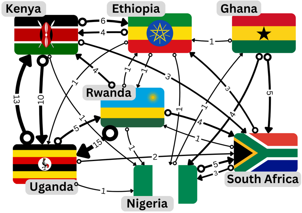
In this lesson we will work with a small network built from Wikipedia pages of Ethiopia, Ghana, Kenya, Nigeria, Rwanda, South Africa and Uganda – chosen for being the home countries of the African members of the Kujenga team. These pages represent a tiny part of the internet but the principles we will learn can be applied to networks of any size. See the video below where Amy introduces our tiny internet.

We represent our network of Wikipedia pages as a directed graph where each node represents a country, shown as labeled country flags in the video. In order to construct the connections between nodes in the graph we check on each country’s page for links to the other 6 countries. For example, in the first paragraph of the page for Ethiopia we read:

Ethiopia, officially the Federal Democratic Republic of Ethiopia, is a landlocked country located in the Horn of Africa region of East Africa. It shares borders with Eritrea to the north, Djibouti to the northeast, Somalia to the east, Kenya to the south, South Sudan to the west, and Sudan to the northwest.

Here we see a link to Kenya, meaning we should count this as a connection from Ethiopia to Kenya. We represent this connection as a directed edge in the graph, shown by an arrow pointing from Ethiopia to Kenya. The weight of each edge, shown as a number next to the edge, counts the total number of links from page A to page B, in this case, there are a total of 4 links from from Ethiopia’s page to Kenya’s.

Note

Wikipedia is a dynamic website and the links between pages can change over time, the network we are using is a snapshot of the Wikipedia pages taken in November 2024. You may want to update this network or even add your home country if is not already included.

Food for Thought

As Amy mentions in the video, use your intuitive understanding of the problem to predict which countries’ pages you think will have a high (or low) ranking.

The methods

We have seen a graphical representation of a network in The problem but in order to use the PageRank algorithm we will need to represent the network mathematically as a matrix. In the following section, we will learn how to work with matrices as well as some basic concepts of linear algebra. The most useful concepts for understanding PageRank will be the notions of an eigenvector and eigenvalue of a matrix which we cover in Eigenvalues and eigenvectors of a matrix.

The Mathematics of the PageRank algorithm

The PageRank algorithm can be understood as modeling the behavior of a “random surfer” navigating the internet. This surfer either clicks on a link on the current page or occasionally gets bored and jumps to a completely random page. The PageRank score of a page represents the long-term probability that this random surfer will end up on that particular page.

Preliminaries

Let’s break down the process mathematically. In this section we will define the key variables and concepts needed to understand the PageRank algorithm.

The PageRank Vector (R):

\[\begin{split}\mathbf{R} = \begin{pmatrix} r_1 \\ r_2 \\ \vdots \\ r_N \end{pmatrix}.\end{split}\]

This vector R represents the PageRank scores for all N=7 pages in the graph. Each element r_i is the PageRank score of the i-th page. Initially, these scores can be set equally, for example, r_i = 1/N for all i.

The Transition Matrix (M):

\[\begin{split}M_{ij} = \begin{cases} 1/L_j^{\text{out}}, & \text{if } j \text{ links to } i \\ 0, & \text{otherwise.} \end{cases}\end{split}\]

This matrix M (often called the hyperlink matrix or transition matrix) encodes the link structure of the network. We use the following notation:

• L_j^out is the total number of outgoing links from page j.

• M_ij represents the probability of transitioning from page j to page i by following some specific link.

  • If page j links to page i, the probability of following a specific link from j to i is 1/L_j^out , assuming the surfer chooses randomly among all outgoing links.

  • If there is no link from j to i, then M_ij = 0.

The Iterative Update Rule

\[\mathbf{R}(t + 1) = d\mathbf{M}\mathbf{R}(t) + \frac{1-d}{N} \mathbf{1}\]

This is the core formula for calculating PageRank iteratively. In the equation above:

• R(t) is the PageRank vector at iteration t, and R(t+1) is the vector at the next iteration.

• d is the “damping factor” (typically around 0.85). It represents the probability that the random surfer will continue following links (as opposed to jumping to a random page). In practice, this is important to handle “dangling nodes”, nodes with no outgoing links, i.e. L_j^out = 0.

MR(t) calculates how the PageRank scores at time t, R(t), are distributed across the network by following links. Element i of the resulting vector is the sum of PageRank contributions from all pages j that link to page i. Therefore, dMR(t) is the portion of the PageRank score derived from surfers following links.

The probability that the surfer gets bored and jumps to a random page is 1-d. Therefore, (1-d)/N is the probability of landing on any specific page during a random jump (assuming N pages total). Let 1 be a column vector of size N containing all ones. Then, (1-d)/N 1 represents the PageRank score distributed equally among all pages due to the random jump behavior. This term ensures that all pages receive some minimal rank and helps the algorithm converge. This is important for dealing with nodes with no outgoing links, i.e. L_j^out = 0, as mentioned earlier, or disconnected parts of the graph.

Convergence

The iterative update process is repeated until the PageRank vector R stabilizes. Convergence is achieved when

\[\mathbf{R}(t + 1) = \mathbf{R}(t).\]

In practice, we check for convergence by monitoring the difference between the PageRank vector in the current iteration R(t+1) and the previous iteration R(t). When the difference is very small (below some predefined threshold), we stop the iterations. The final vector R* represents the stable probability distribution of the random surfer, indicating the relative importance of each page.

Simplified update rule for connected graphs

Looking at the graph representing our network of Wikipedia pages we can see that the graph is “connected”, a technical term meaning there is a path between every pair of distinct nodes ignoring the direction of the edges. Therefore, we do not need to take into account any “dangling nodes”, nodes with no outgoing links L_j^out = 0, or disconnected parts of the graph.

Using this observation we can simplify the update rule by setting d = 1. This means that the random surfer will always follow a link and never jump to a random page. The update rule becomes:

\[\mathbf{R}(t + 1) = \frac{1}{\lambda} \mathbf{M}\mathbf{R}(t)\]

Here we introduce a normalization factor \(\lambda\). This normalization ensures that all PageRank scores (element of the vector R) sum to a constant value.

Assuming the algorithm has converged, R(t + 1) = R(t), you might already recognize the resemblance to the eigenvalue equation:

\[\mathbf{M}\mathbf{R} = \lambda \mathbf{R}\]

If not don’t worry, we will cover the details in the section Eigenvalues and eigenvectors of a matrix.

In the video below Amy discusses the theory above and shows the results of applying the simplified update rule iteratively. You will see how to implement this yourself in the section Constructing the transition matrix M and Simulating PageRank.

Food for Thought

It turned out that Nigeria had the highest PageRank and Kenya and Uganda the lowest. Did this match your expectations based on the network shown in section The problem.

Working with matrices in Python

NumPy (Numerical Python) is the fundamental package for scientific computing in Python. It provides a powerful N-dimensional array object and tools for working with these arrays. We’ll use NumPy arrays to represent vectors (1D arrays) and matrices (2D arrays).

Importing NumPy

NumPy is a third-party library, so you need to install it separately. If you are using Google Colab, it is already included. To load NumPy with the alias np, you can use the following command:

import numpy as np

Defining a vector (1D Arrays)

A vector can be thought of as a list of numbers. In NumPy, you create it using np.array() with a Python list:

my_list = [1, 2, 3]
my_vector = np.array(my_list)

print("My Vector:")
print(my_vector)

My Vector:
[1 2 3]

Check its shape (dimensions) Output: (3,) indicates a 1D array with 3 elements

print("Vector shape:", my_vector.shape)

Vector shape: (3,)

Creating Matrices (2D Arrays)

A matrix is like a grid of numbers (rows and columns). You create it using np.array() with a list of lists, where each inner list is a row:

my_lists = [[1, 2, 3], [4, 5, 6]]
my_matrix = np.array(my_lists)

print("\nMy Matrix:")
print(my_matrix)

My Matrix:
[[1 2 3]
 [4 5 6]]

Check its shape (rows, columns) Output: (2, 3) indicates 2 rows and 3 columns

print("Matrix shape:", my_matrix.shape)

Matrix shape: (2, 3)

Create a square matrix (same number of rows and columns)

square_matrix = np.array([[9, 8], [7, 6]])
print("\nSquare Matrix:")
print(square_matrix)
print("Square Matrix shape:", square_matrix.shape)

Square Matrix:
[[9 8]
 [7 6]]
Square Matrix shape: (2, 2)

Basic Operations

NumPy makes operating on vectors and matrices straightforward. Element-wise Operations: Standard arithmetic operators (+, -, *, /) often work element-by-element if the shapes are compatible.

vec1 = np.array([1, 2, 3])
vec2 = np.array([4, 5, 6])
mat1 = np.array([[1, 1], [2, 2]])
mat2 = np.array([[3, 3], [4, 4]])

Vector addition (element-wise)

print("\nVector Addition:", vec1 + vec2)  # Output: [5 7 9]

Vector Addition: [5 7 9]

Matrix addition (element-wise)

print("Matrix Addition:\n", mat1 + mat2)

Matrix Addition:
 [[4 4]
 [6 6]]

Scalar multiplication (multiply every element by a number)

print("Scalar Multiplication (Vector):", 3 * vec1)  # Output: [3 6 9]
print("Scalar Multiplication (Matrix):\n", 2 * mat1)

Scalar Multiplication (Vector): [3 6 9]
Scalar Multiplication (Matrix):
 [[2 2]
 [4 4]]

Dot Product / Matrix Multiplication: This is different from element-wise multiplication (*). It’s the standard mathematical operation. Use np.dot() or the @ operator.

vec1 = np.array([1, 2, 3])
vec2 = np.array([4, 5, 6])

Vector dot product (sum of element-wise products)

dot_product = np.dot(vec1, vec2)  # 1*4 + 2*5 + 3*6 = 4 + 10 + 18 = 32
print("Vector Dot Product:", dot_product)

Vector Dot Product: 32

Or using the @ operator

dot_product_alt = vec1 @ vec2
print("Vector Dot Product (@):", dot_product_alt)

Vector Dot Product (@): 32

Matrix multiplication

mat1 = np.array([[1, 2], [3, 4]])  # 2x2 matrix
mat2 = np.array([[5, 6], [7, 8]])  # 2x2 matrix
matrix_product = np.dot(mat1, mat2)
print("Matrix Multiplication:\n", matrix_product)

Matrix Multiplication:
 [[19 22]
 [43 50]]

Or using the @ operator

matrix_product_alt = mat1 @ mat2
print("Matrix Multiplication (@):\n", matrix_product_alt)

Matrix Multiplication (@):
 [[19 22]
 [43 50]]

vec3 = np.array([10, 20])  # 1x2 vector
# Matrix-vector multiplication
mat_vec_product = np.dot(mat1, vec3)  # Note: Treats vec3 as a column vector here
print("Matrix-Vector Multiplication:", mat_vec_product)

Matrix-Vector Multiplication: [ 50 110]

Or using the @ operator

mat_vec_product_alt = mat1 @ vec3
print("Matrix-Vector Multiplication (@):", mat_vec_product_alt)

Matrix-Vector Multiplication (@): [ 50 110]

Note

Simple multiplication \(*\) is element-wise, not matrix multiplication!

print("Element-wise Matrix Multiplication (NOT dot product):\n", mat1 * mat2)

Element-wise Matrix Multiplication (NOT dot product):
 [[ 5 12]
 [21 32]]

Rule for A @ B: The number of columns in A must equal the number of rows in B. Transpose: Swaps rows and columns. Use the .T attribute.

matrix = np.array([[1, 2, 3], [4, 5, 6]])
print("\nOriginal Matrix:\n", matrix)
print("Transposed Matrix:\n", matrix.T)
print("Original shape:", matrix.shape)  # Output: (2, 3)
print("Transposed shape:", matrix.T.shape)  # Output: (3, 2)

Original Matrix:
 [[1 2 3]
 [4 5 6]]
Transposed Matrix:
 [[1 4]
 [2 5]
 [3 6]]
Original shape: (2, 3)
Transposed shape: (3, 2)

Accessing Elements

You can access elements using zero-based indexing, similar to Python lists. For matrices, use [row, column].

vector = np.array([10, 20, 30, 40])
matrix = np.array([[1, 2], [3, 4]])

Get the first element of the vector (index 0)

print("\nVector element [0]:", vector[0])  # Output: 10

Vector element [0]: 10

Get the element at row 1, column 0 of the matrix

print("Matrix element [1, 0]:", matrix[1, 0])  # Output: 3

Matrix element [1, 0]: 3

Get an entire row (e.g., row 0)

print("Matrix row [0]:", matrix[0])  # Output: [1 2]

Matrix row [0]: [1 2]

Get an entire column (e.g., column 1) using slicing ‘:’

print("Matrix column [:, 1]:", matrix[:, 1])  # Output: [2 4]

Matrix column [:, 1]: [2 4]

Constructing the transition matrix M

The transition matrix M, given in section Preliminaries, has elements

\[\begin{split}M_{ij} = \begin{cases} 1/L_j^{\text{out}}, & \text{if } j \text{ links to } i \\ 0, & \text{otherwise} \end{cases}\end{split}\]

where L_j^out is the total number of outgoing links from page j.

From the network shown in section The problem we can count up the number of outgoing links for each country and summarize them in a table.

Number of outgoing links for each country (L_j^out)

Country	Number of outgoing links
ZA	7
GH	10
NG	6
RW	25
UG	21
KE	20
ET	7

We can again use the network shown in section The problem to check if if there is a link from country j to country i. For example, we can see that there is a link from Ethiopia to Kenya but not from Ethiopia to South Africa. Combining these two pieces of information we can construct the transition matrix M as shown in the table below.

PageRank matrix elements

	ZA	GH	NG	RW	UG	KE	ET
ZA	0	1/10	1/6	1/25	1/21	1/20	0
GH	0	0	1/6	0	0	0	0
NG	1/7	1/10	0	1/25	1/21	1/20	1/18
RW	1/7	0	0	0	1/21	0	1/18
UG	0	0	0	1/25	0	1/20	1/18
KE	0	0	0	1/25	1/21	0	1/18
ET	1/7	1/10	0	1/25	0	1/20	0

This table can be translated into Python code as a NumPy array:

M = np.array(
    [
        [0, 1 / 10, 1 / 6, 1 / 25, 1 / 21, 1 / 20, 0],
        [0, 0, 1 / 6, 0, 0, 0, 0],
        [1 / 7, 1 / 10, 0, 1 / 25, 1 / 21, 1 / 20, 1 / 18],
        [1 / 7, 0, 0, 0, 1 / 21, 0, 1 / 18],
        [0, 0, 0, 1 / 25, 0, 1 / 20, 1 / 18],
        [0, 0, 0, 1 / 25, 1 / 21, 0, 1 / 18],
        [1 / 7, 1 / 10, 0, 1 / 25, 0, 1 / 20, 0],
    ]
)

print(M)

[[0.         0.1        0.16666667 0.04       0.04761905 0.05
  0.        ]
 [0.         0.         0.16666667 0.         0.         0.
  0.        ]
 [0.14285714 0.1        0.         0.04       0.04761905 0.05
  0.05555556]
 [0.14285714 0.         0.         0.         0.04761905 0.
  0.05555556]
 [0.         0.         0.         0.04       0.         0.05
  0.05555556]
 [0.         0.         0.         0.04       0.04761905 0.
  0.05555556]
 [0.14285714 0.1        0.         0.04       0.         0.05
  0.        ]]

Food for Thought

If a new link between two pages were added or even a whole new page, how would with change the matrix M? Does such a change to M represent a large or small computational cost? Consider this in a real-world context where the number of pages (nodes in the network) could be extremely large.

Simulating PageRank

Let’s choose an initial PageRank vector R(0) and apply the update rule iteratively until convergence.

R = np.array([1, 1, 1, 1, 1, 1, 1]) * 100 / 7  # Initial PageRank vector
print("Initial PageRank vector R(0):", R)

Initial PageRank vector R(0): [14.28571429 14.28571429 14.28571429 14.28571429 14.28571429 14.28571429
 14.28571429]

Create a variable t to keep track of the number of iterations performed

t = 0  # Iteration counter
print("Iteration:", t)

Iteration: 0

Create a vector with the county codes which will be used to label the PageRank vector

countries = ["ZA", "GH", "NG", "RW", "UG", "KE", "ET"]
print("Countries:", countries)

Countries: ['ZA', 'GH', 'NG', 'RW', 'UG', 'KE', 'ET']

Apply the update rule

R = np.dot(M, R)  # Update PageRank vector using matrix multiplication
R = R / np.sum(R) * 100  # Normalize the PageRank vector to sum to 100
print(
    f"Updated PageRank vector R({t+1}):\n",
    "\n ".join([f"{c}: {r:.2f}" for c, r in zip(countries, R)]),
)
t += 1  # Increment iteration counter

Updated PageRank vector R(1):
 ZA: 21.57
 GH: 8.89
 NG: 23.26
 RW: 13.12
 UG: 7.76
 KE: 7.64
 ET: 17.76

Run the cell above multiple times to see how the PageRank vector converges. If you want to start again be sure to rerun all the cells in the Simulating PageRank section to avoid unexpected behavior.

Food for Thought

If you run the cell above multiple times you will see that the PageRank vector converges to a stable value. How many iterations does it take to converge? Do you think this is a reasonable number of iterations for a real-world application? What happens if you choose a different initial PageRank vector? Does it converge to the same value?

Eigenvalues and eigenvectors of a matrix

In the video below Amandine and Amy give a brief introduction to eigenvalues and eigenvectors and how they are applied in the context of the PageRank algorithm.

Let’s summarize the mathematics shown in the video. The N-by-N matrix M has N eigenvectors \(\mathbf{v}_i\) which obey the equation:

\[\mathbf{M}\mathbf{v}_i = \lambda_i \mathbf{v}_i\]

where \(\lambda\)_i is the eigenvalue associated with the eigenvector \(\mathbf{v}_i\).

The eigenvalue equation states that when the matrix M acts on the eigenvector \(\mathbf{v}_i\), it scales the vector by a factor of \(\lambda_i\) without changing its direction.

Let’s use Python to compute the eigenvalues and the corresponding eigenvectors of the transition matrix M. We will use the numpy.linalg.eig() function to compute the eigenvalues and eigenvectors of a matrix.

eigenValues, eigenVectors = np.linalg.eig(M)
print("Eigenvalues:", eigenValues)

Eigenvalues: [ 0.29255874+0.j         -0.1132207 +0.0347069j  -0.1132207 -0.0347069j
  0.03257219+0.j         -0.02452311+0.03602166j -0.02452311-0.03602166j
 -0.0496433 +0.j        ]

Note that some of the eigenvalues are complex, e.g. \(0.02227925-0.04471056i\) (in Python “j” is used to represent the imaginary unit).

Let’s get the index of the largest eigenvalue by first getting a list of the indices of the sorted eigenValues:

idx = eigenValues.argsort()[::-1]  # eigenValues in descending order

print(idx)

[0 3 4 5 6 1 2]

Now let’s replace the eigenValues and eigenVectors with the sorted versions

eigenValues = eigenValues[idx]
eigenVectors = eigenVectors[:, idx]

print("Sorted Eigenvalues:", eigenValues)

Sorted Eigenvalues: [ 0.29255874+0.j          0.03257219+0.j         -0.02452311+0.03602166j
 -0.02452311-0.03602166j -0.0496433 +0.j         -0.1132207 +0.0347069j
 -0.1132207 -0.0347069j ]

The largest eigenvalue is the first element of the sorted eigenValues array. The corresponding eigenvector is the first column of the sorted eigenVectors array.

eigenvalue0 = eigenValues[0]
eigenvector0 = eigenVectors[:, 0]
print("Largest Eigenvalue:", eigenvalue0)
print("Corresponding Eigenvector:", eigenvector0)

Largest Eigenvalue: (0.2925587369323658+0j)
Corresponding Eigenvector: [0.51030388+0.j 0.30519189+0.j 0.53571932+0.j 0.35611479+0.j
 0.15671107+0.j 0.15562185+0.j 0.42878715+0.j]

Check that the eigenvalue equation holds:

RHS = np.dot(M, eigenvector0)  # Right had side of the eigenvalue equation
print("M @ eigenvector0:")
print(RHS)
LHS = eigenvalue0 * eigenvector0  # Left hand side of the eigenvalue equation
print("eigenvalue0 * eigenvector0:")
print(LHS)
print("Euclidean distance (should be close to zero):")
print(np.sqrt(np.sum((RHS - LHS) ** 2)))

M @ eigenvector0:
[0.14929386+0.j 0.08928655+0.j 0.15672937+0.j 0.10418449+0.j
 0.04584719+0.j 0.04552853+0.j 0.12544543+0.j]
eigenvalue0 * eigenvector0:
[0.14929386+0.j 0.08928655+0.j 0.15672937+0.j 0.10418449+0.j
 0.04584719+0.j 0.04552853+0.j 0.12544543+0.j]
Euclidean distance (should be close to zero):
(2.939012725487379e-16+0j)

In the final video Amandine will briefly take you through the computation of the eigenvalues and eigenvalues of the transition matrix M including how to sort them to extract the largest eigenvalue and its corresponding eigenvector.

Directly computing the PageRank scores

Does this help us predict the PageRank scores? Let’s normalize “eigenvector0” and check that the values correspond to the PageRank scores obtained using the iterative method applied in the section Simulating PageRank.

eigenvector0_normalized = eigenvector0 / np.sum(eigenvector0) * 100
print(
    f"Normalized largest eigenvector:\n",
    "\n ".join([f"{c}: {r:.2f}" for c, r in zip(countries, eigenvector0_normalized)]),
)

Normalized largest eigenvector:
 ZA: 20.84+0.00j
 GH: 12.46+0.00j
 NG: 21.88+0.00j
 RW: 14.54+0.00j
 UG: 6.40+0.00j
 KE: 6.36+0.00j
 ET: 17.51+0.00j

What about the other eigenvalues and eigenvectors? Why do we only need to consider the eigenvalue with the largest magnitude and its corresponding eigenvector? It turns out that the eigenvalue with the largest magnitude is the only one that matters for the PageRank algorithm.

Eigenvectors corresponding to distinct eigenvalues are always linearly independent. You can verify that this is the case for our transition matrix M. Consequently, it is possible to rewrite any initial state R(0) as a linear combination of the eigenvectors v_i of M,

\[\mathbf{R}(0) = \sum_{i=1}^N a_i \mathbf{v}_i.\]

The PageRank vector R(1) at iteration \(t=1\) can be expressed as a linear combination of the eigenvectors of M as:

\[\mathbf{R}(1) =\mathbf{M} \mathbf{R}(0) = \sum_{i=1}^N a_i \mathbf{M}\mathbf{v}_i = \sum_{i=1}^N a_i \lambda_i\mathbf{v}_i\]

Applying M t times you can convince yourself that

\[\mathbf{R}(t) = \sum_{i=1}^N a_i \mathbf{M}^t\mathbf{v}_i = \sum_{i=1}^N a_i \lambda_i^t\mathbf{v}_i,\]

where \(a_i\) depend on the initial chose of R(0). Assuming that the eigenvalues are labeled so that \(|\lambda_1| > |\lambda_2| \geq |\lambda_3| \geq ... \geq |\lambda_N|\), the term \(\lambda_1^t a_1 \mathbf{v}_1\) will dominate the sum as t increases, and the PageRank vector will converge to a multiple of the eigenvector corresponding to the largest eigenvalue.

Exercises

Complete the following exercises to deepen your understanding of the PageRank algorithm and its behavior under different conditions.

Exercise 1: The “Digital Influencer” Challenge

In this exercise, you will add a additional country to the existing network to see how it affects the rankings.

1. Create a new 8-by-8 matrix called M_extended.

2. Copy the values from the original 7-by-7 matrix M into the top-left corner of your new matrix.

3. Add an additional (fictional) country as the 8th node (index 7).

4. Outgoing Links: You have a “budget” of 3 links. Choose 3 countries from the original list for your country to link to.

5. Incoming Links: Assume that Nigeria (NG) and South Africa (ZA) are impressed by your page and each add a link to your country.

6. Run the iterative simulation. Where does the added country rank? Use the simplified update rule described in section The Iterative Update Rule with d = 1.

7. How does linking to high- and low-ranked countries affect your country’s PageRank score?

Tip

When Nigeria and South Africa add a link to you, their total number of outgoing links (\(L_j^{out}\)) increases, so you will need to update the matrix accordingly.

Exercise 2: The “Boredom Factor” Sensitivity Test

The damping factor \(d\) represents the probability that a surfer continues clicking links. If \(d=0\), the surfer is “completely bored” and only ever jumps to random pages. Using the full update rule described in section The Iterative Update Rule:

1. Write a loop that calculates the final PageRank scores for all 7 countries for different values of \(d\), ranging from 0.0 to 1.0 in steps of 0.05.

2. Use matplotlib.pyplot to generate a plot where the x-axis is the value of \(d\) and the y-axis is the PageRank score.

3. Plot a separate curve for each country.

4. Comment on the sensitivity of the PageRank scores to changes in the damping factor.

YOU CAN SUBMIT YOUR ASSIGNMENT HERE