The SEIR model

Now you should study a model yourself! Download the page as a Python notebook and fill in the missing code according to the instructions.

In the SEIR model, there is an additional class for people exposed (but not yet infective). The equations are now,

\[\begin{aligned} \frac{dS}{dt} & = & - \beta S I \ \frac{dE}{dt} & = & \beta S I - \delta E\ \frac{dI}{dt} & = & \delta E - \gamma I \ \frac{dR}{dt} & = & \gamma I \end{aligned}\]

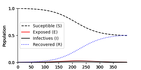
Simulating the model

Assume that \(\gamma=1/7\) and \(\beta=1/5\). Write code to draw a graph of \(I(t)\) as a function of time (\(t\)) for the cases in which (on average) a person is exposed for 1, 5 and respectively 9 days before they are infected. Assume that \(S(0)=999/1000\), \(E(0)=0\) and \(I(0)=1/1000\).

import numpy as np
import matplotlib.pyplot as plt
from pylab import rcParams
import matplotlib
rcParams['figure.figsize'] = 12/2.54, 6/2.54
matplotlib.font_manager.FontProperties(family='Helvetica',size=11)
from scipy import integrate

# Parameter values
beta = 1/5
gamma = 1/7

timesteps=400

# Set up the equations here
def dXdt(X, t=0):
    return np.array([  - beta*X[0]*X[2] ,              #Susceptible X[0] is S
                      beta*X[0]*X[2]   - delta*X[1],    #Exposed X[1] is I
                      delta*X[1]   - gamma*X[2],      #Infectives X[2] is I
                      gamma*X[2]])                      #Recovered X[3] is R


def plotEpidemicOverTime(ax,S,E,I,R):

    ax.plot(t, S, '--',color='k', label='Suceptible (S)')
    ax.plot(t, E  , '',color='r', label='Exposed (E)')
    ax.plot(t, I  , '-',color='k', label='Infectives (I)')
    ax.plot(t, R  , ':',color='b', label='Recovered (R)')
    ax.legend(loc='best')
    ax.set_xlabel('Time: t')
    ax.set_ylabel('Population')
    ax.spines['top'].set_visible(False)
    ax.spines['right'].set_visible(False)
    ax.set_xticks(np.arange(0,timesteps,step=50))
    ax.set_yticks(np.arange(0,1.01,step=0.5))
    ax.set_xlim(0,timesteps)
    ax.set_ylim(0,1)

t = np.linspace(0, timesteps,  1000)               # time
X0 = np.array([0.999, 0.000, 0.001,0.0000])      # initially 99.9% are uninfected

# Set delta here
for delta in np.array([1,1/5,1/9]):
    X = integrate.odeint(dXdt, X0, t) # uses a Python package to simulate the interactions
    S, E, I, R = X.T
    fig,ax=plt.subplots(num=1)
    plotEpidemicOverTime(ax,S,E,I,R)
    plt.show()

/Users/davidsumpter/Documents/GitHub/Kujenga/course/lessons/lesson2/plot_SEIR.py:80: UserWarning: FigureCanvasAgg is non-interactive, and thus cannot be shown
  plt.show()

Does \(\delta\) have a large effect on the final number of people infected? Add a text box and explain your answer below.

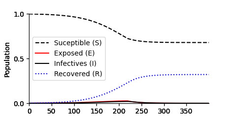
Introducing restrictions

The helath authority decide to introduce restrictions when a threshold \(I_T`% of the population are infected. With restrictions :math:\)beta=1/10` and without them \(\beta=1/5\). The other paramters are \(\gamma=1/7\) and \(\delta=1/3\). Investigate the consequences of that decision for various values of \(\delta\), i.e. simulate the spread,with \(\beta=1/5\) until \(I(t)=I_T\) and then with \(\beta=1/10\). Make plots of \(R(t)\) for different \(T\) values

t1 = np.linspace(0, timesteps,  1000)               # time
X0 = np.array([0.999, 0.000, 0.001,0.0000])      # initially 99.9% are uninfected

# Set delta here
for IT in np.array([0.005,0.01,0.02]):
    beta = 1/5
    X1 = integrate.odeint(dXdt, X0, t1) # uses a Python package to simulate the interactions
    S, E, I, R = X1.T
    ind = (I>=IT).nonzero()[0]
    onepercent=int(ind[0])
    New_X0 = X1[onepercent,:]
    X = X1[:onepercent,:]
    t = t1[:onepercent]
    t2 = np.linspace(t1[onepercent], timesteps,  1000)

    beta = 1/10
    X2 = integrate.odeint(dXdt, New_X0, t2) # uses a Python package to simulate the interactions
    X = np.concatenate((X, X2), axis=0)
    t = np.concatenate((t, t2), axis=0)
    S, E, I, R = X.T
    fig,ax=plt.subplots(num=1)
    plotEpidemicOverTime(ax,S,E,I,R)
    plt.show()

/Users/davidsumpter/Documents/GitHub/Kujenga/course/lessons/lesson2/plot_SEIR.py:126: UserWarning: FigureCanvasAgg is non-interactive, and thus cannot be shown
  plt.show()

Code help

The following command will help you find then \(I(t) \geq 0.01\)

I = np.array([0.001, 0.0025, 0.005, 0.01, 0.02, 0.05])
ind = (I>=0.01).nonzero()[0]
onepercent=int(ind[0])
print('Infectives became 1 percent at time %d'% onepercent)

Infectives became 1 percent at time 3

The following code concatenates two arrays

X1 = np.array([[1, 2],[2,3],[3,6]])
X2 = np.array([[3, 8],[4,9],[5,12]])

X = np.concatenate((X1, X2), axis=0)

print('Concatinated matrix:\n')
print(X)

Concatinated matrix:

[[ 1  2]
 [ 2  3]
 [ 3  6]
 [ 3  8]
 [ 4  9]
 [ 5 12]]

Conclusions

Add a text box below and describe (in words) how \(\delta\) affects the outcome.