Note
Click here to download the full example code
The social epidemic
In this section we go on to solve some more differential equations which describe rules of interaction. Here I assume you have already worked through and understood the section on predator prey models.
In the book I first introduce the SIR model of disease spread, by looking at infections.

Then I discuss recoveries.

Let’s turn these rules of interaction in to differential equations and analyse how they describe disease spread.
The SIR model
In terms of differential equations, the rate of change of susceptible individuals is
and the rate of change of infectives is
The constant \(b\) is the rate of contact between people and \(c\) is the rate of recovery. We can also write down an equation for recovery as follows,
In this model \(S\), \(I\) and \(R\) are proportions of the population. Summing them up gives \(S+I+R=1\), since everyone in the popultaion is either susceptible, infective or recovered.
Let’s now solve these equations numerically. We start by importing the libraries we need from Python.
import numpy as np
import matplotlib.pyplot as plt
import matplotlib
from pylab import rcParams
matplotlib.font_manager.FontProperties(family='Helvetica',size=11)
rcParams['figure.figsize'] = 9/2.54, 9/2.54
from scipy import integrate
Now we define the model. This code creates a function which we can use to simulate differential equations (1) and (2). We also define the parameter values. You can change these to see how changes to the paramaters leads to changes in the outcome of the model.
# Parameter values
b = 3.5
c = 1

# Differential equation
def dXdt(X, t=0):
    # Growth rate of fox and rabbit populations.
    return np.array([  - b*X[0]*X[1] ,      #Susceptible X[0] is S
                      b*X[0]*X[1]   - c*X[1],      #Infectives X[1] is I
                      c*X[1]])                     #Recovered X[2] is R
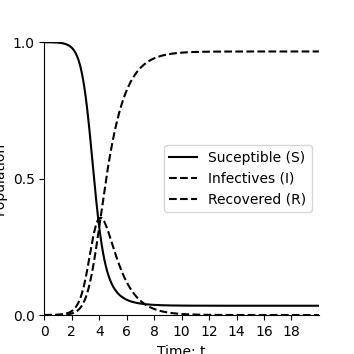
We solve the equations numerically and plot solution over time.
def plotEpidemicOverTime(ax,S,I,R):

    ax.plot(t, S, '-',color='k', label='Suceptible (S)')
    ax.plot(t, I  , '--',color='k', label='Infectives (I)')
    ax.plot(t, R  , '--',color='k', label='Recovered (R)')
    ax.legend(loc='best')
    ax.set_xlabel('Time: t')
    ax.set_ylabel('Population')
    ax.spines['top'].set_visible(False)
    ax.spines['right'].set_visible(False)
    ax.set_xticks(np.arange(0,20,step=2))
    ax.set_yticks(np.arange(0,1.01,step=0.5))
    ax.set_xlim(0,20)
    ax.set_ylim(0,1)


t = np.linspace(0, 20,  1000)               # time
X0 = np.array([0.9999, 0.0001,0.0000])      # initially 99.99% are uninfected
X = integrate.odeint(dXdt, X0, t)           # uses a Python package to simulate the interactions
S, I, R = X.T
fig,ax=plt.subplots(num=1)
plotEpidemicOverTime(ax,S,I,R)
plt.show()

# .. admonition:: Think yourself!
#
#     When :math:`b=1`, for what values of :math:`c` does the number of infectives
#     always decrease? Try changing the initial number of infectives to :math:`0.5`.
#     Now find values of :math:`c` where the number of infectives
#     always decreases?
/Users/davidsumpter/Documents/GitHub/Kujenga/course/lessons/lesson2/plot_socialepidemic.py:107: UserWarning: FigureCanvasAgg is non-interactive, and thus cannot be shown
  plt.show()
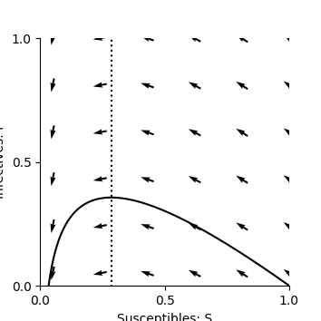
As with the precator prey model we can find the equilibria where the rate at which people become infected equals the rate at which they recover by solving
This occurs either when \(I=0\) (no-one has the disease) or when \(S=c/b\). We can now plot these equilibrium on the phase plane
def plotPhasePlane(ax,S,I):
    ax.plot(S, I, '-',color='k')
    ax.set_xlabel('Susceptibles: S')
    ax.set_ylabel('Infectives: I')
    ax.spines['top'].set_visible(False)
    ax.spines['right'].set_visible(False)
    ax.set_xticks(np.arange(0,1.01,step=0.5))
    ax.set_yticks(np.arange(0,1.01,step=0.5))
    ax.set_ylim(0,1)
    ax.set_xlim(0,1)

def drawArrows(ax,dXdt):
    x = np.linspace(0.05, 1 ,6)
    y = np.linspace(0.05, 1, 6)
    X , Y  = np.meshgrid(x, y)
    dX, dY, dZ = dXdt([X, Y,1-X-Y])
    #Make in to unit vectors.
    M = np.hypot(dX,dY)
    dX = dX/M
    dY = dY/M
    ax.quiver(X, Y, dX, dY, pivot='mid')

fig,ax=plt.subplots(num=1)
ax.plot([c/b,c/b],[-100,100],linestyle=':',color='k')
plotPhasePlane(ax,S,I)
drawArrows(ax,dXdt)
plt.show()
/Users/davidsumpter/Documents/GitHub/Kujenga/course/lessons/lesson2/plot_socialepidemic.py:157: UserWarning: FigureCanvasAgg is non-interactive, and thus cannot be shown
  plt.show()
The solution to \(S=c/b\) is known as herd immunity. When \(S>c/b\) then the number of infectives increase. So when \(S=0.9999\) then if \(b>0.9999c\) then the infection increases and when \(b<0.9999c\) then the infection decreases. Simiarly, when \(S=0.5`then if :math:`b>0.5c\) then the infection increases and it decreases when \(b<0.5c\).
Social recovery
For many social behaviours, it isn’t just the adoption of a fad or a news cycle that is contagious, but also the way in which we recover. When we get a cold, flu or Covid-19, the best thing to do is to go home, rest and not spread the virus. Spending time with people who have already been ill doesn’t help us recover more quickly (even if their sympathy might help us feel a bit better). Recovery is independent between individuals. In the book, I look at social recovery, when it depends on how many are recovered.
In terms of differential equations, the rate of change of susceptible individuals remains the same as before
but the rate of change of infectives is now
The constant \(b\) is the rate of contact between people and \(c\) is the rate of contact between infectives and recovered individuals. We can also write down an equation for recovery as follows,
In Python these equations are written as follows.
Again, we can find the equilibria where the rate at which people become infected equals the rate at which they recover by solving
This occurs either when \(I=0\) (no-one has the disease) or
when
or, equivalently,
or .. math:
We can now plot these equilibrium on the phase plane