Note
Click here to download the full example code
Rabbits and foxes
In this section we will learn how to write differential equations models to show the rate of change of populatins of predators and prey. We will simulate the model using Python. Then we draw the phase plane for the model, just as Parker does in the book in the image shown below.

Differential equations
In the book, I write Lotka’s equations in the form of chemical reactions, e.g.
This means that an F and R together becomes two F’s. My character from Santa Fe, Professor Parker expalins as follows,

While in Leipzig, A. J. Lotka learnt how chemical reactions can be used to specify the rate of change of populations, i.e. in terms of the derivates above, using an approach, known as the law of mass action. The idea is to think about the rate at which these chemical reactions take place. For the first reaction
We can think of \(a\) as being the rate of reproduction of the rabbits, how many baby rabbits an adult rabbit has per day. So, the rabbits grow according to
This equation denotes the rate of change of \(R\) over time. the top part of the fraction \(dR\) denotes the change in rabbits, \(R\), and the bottom part, \(dt\), denotes the change in time, \(t\).
Differentiation in school
This section is somewhat of an aside, but it might be useful if you have studied differentiation before. I remember that after learning about differentiation in school, I found the form of differential equations above to be a bit strange when I firstencountered it. In school we might have a function that looks like, for example,
then take the derivative to get
This is also a differential equation. It says that the rate of change of \(X\) over time is proportional to time. The difference between equation (3) and (1) is that (3) says that rabbits grow in proportion to time, while (1) says that rabbits grow proportionally to the number of rabbits.
In the case that rabbits grow in proportion to time, then we say that (2) is the solution to equation (3) since it tells us how many rabbits there will be at any point in time. As yet, we haven’t found a solution to equation (1).
I think this is where differential equations can be a bit confusing, because in school we are usually given (2) and asked to find (3). For most differential equations it is the other way round. We are given equation (1) and asked to find the the number of rabbits \(R\) as a function of time.
The solution to equation (3) is in fact,
assuming that \(R(0)=1\) (see here for an explanation of how we get this solution).
In both these cases, we can find an explicit solution for \(R(t)\) in terms of \(t\). By explicit here I mean that if you tell me a value of \(t\), I can put it in to (4) and tell you the number of rabbits. It is not always the case that we can find an explicit solution. Indeed, for most differential equation models we can’t find solutions of this form. This is the case for the rabbits and foxes model which we now look at. We won’t be able to find an explicit mathematical expression for rabbits and foxes at any time, but we can understand the dynamics of rabbits and foxes.
Back to rabbits anf foxes
We have an equation for growth of rabbits, now we need to have equations that include foxes. In chemical reaction form these are,
for foxes eating rabbits and
for foxes dying. Converted to differential equations, the rate of change for rabbits becomes
Similarly, we can write the rate of change of foxes as
Notice that we have a different rate parameter for the death of rabbits (\(b\)) than for the birth of foxes (\(c\)). This is because it takes more than one rabbit to feed a fox and we set the parameters so that \(c<b\).
It may seem strange to treat rabbits and foxes as chemicals. As we all know, two rabbits are needed to produce baby rabbits and when a fox eats a rabbit it doesn’t simply transform it directly in to a new fox, as the chemical equation suggests. Also, in the description above, the grass is not depleted: there is no chemical equation describing how grass is transformed to rabbit poop. But the point of a mathematical model like this is not to be entirely realistic. Rather, it tries to capture the essence of the problem. We want to imagine a big grassy meadow, where the more rabbits there are, the faster the rabbit population grows and the more foxes there are the faster the rabbits are eaten. We will try to understand this abstract problem first, before we make any claims about what happens to real rabbits and real foxes.
Simulating the model
We can use Python to run a numerical simulation of the model.
# Import the libraries we use
import numpy as np
import matplotlib.pyplot as plt
import matplotlib
from pylab import rcParams
matplotlib.font_manager.FontProperties(family='Helvetica',size=11)
rcParams['figure.figsize'] = 14/2.54, 10/2.54
from scipy import integrate
We start by defining the model. This code creates a function which we can use to simulate differential equations (5) and (6).
# Differential equation
def dXdt(X, t=0):
    # Growth rate of fox and rabbit populations.
    return np.array([ a*X[0]        - b*X[0]*X[1] ,      #Rabbits X[0] is R
                      c*X[0]*X[1]   - d*X[1]])           #Foxes X[1] is F
Next we define the parameter values. You can change these to see how changes to the paramaters leads to changes in the outcome of the model.
# Parameter values
a = 5
b = 1
c = 0.15
d = 1
Now we solve the equations numerically
t = np.linspace(0, 20, 1000) # time
X0 = np.array([10, 2]) # initially 10 rabbits and 2 foxes
X = integrate.odeint(dXdt, X0, t)
R, F = X.T
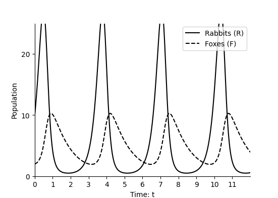
fig,ax=plt.subplots(num=1)
ax.plot(t, R, '-',color='k', label='Rabbits (R)')
ax.plot(t, F , '--',color='k', label='Foxes (F)')
ax.legend(loc='best')
ax.set_xlabel('Time: t')
ax.set_ylabel('Population')
ax.spines['top'].set_visible(False)
ax.spines['right'].set_visible(False)
ax.set_xticks(np.arange(0,12,step=1))
ax.set_yticks(np.arange(0,50,step=10))
ax.set_xlim(0,12)
ax.set_ylim(0,25)
plt.show()
/Users/davidsumpter/Documents/GitHub/Kujenga/course/lessons/lesson2/plot_rabbitsandfoxes.py:211: UserWarning: FigureCanvasAgg is non-interactive, and thus cannot be shown
  plt.show()
First the rabbit populations grow, because there are only two foxes. But this leads to an increase in foxes. Once the population of foxes is sufficiently large, they then start reducing rabbit populations and they die out. Then, when there are few rabbits left, the foxes start to die out too, allowing the rabbit population to grow again.
Think yourself!
Download the code and run it. Try changing the paramater values above. Making \(a\) larger, for example, means the rabbit population grows faster.
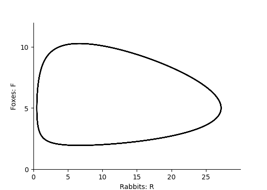
Visualising the cycle
In the figure above, we show how foxes and rabbits change over time. We can also plot how they change relative to each other (a so called phase plane). For the numerical simulations we do this as follows:
def plotPhasePlane(ax,R,F):
    ax.plot(R, F, '-',color='k')
    ax.set_xlabel('Rabbits: R')
    ax.set_ylabel('Foxes: F')
    ax.spines['top'].set_visible(False)
    ax.spines['right'].set_visible(False)
    ax.set_xticks(np.arange(0,30,step=5))
    ax.set_yticks(np.arange(0,20,step=5))
    ax.set_ylim(0,12)
    ax.set_xlim(0,30)


fig,ax=plt.subplots(num=1)
plotPhasePlane(ax,R,F)
plt.show()
/Users/davidsumpter/Documents/GitHub/Kujenga/course/lessons/lesson2/plot_rabbitsandfoxes.py:249: UserWarning: FigureCanvasAgg is non-interactive, and thus cannot be shown
  plt.show()
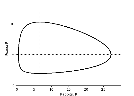
Finding the equilibrium
In order to better understand this cycle we look at the equilibria (the steady states) where the rate at which rabbits are born equals the rate at which they die. We can find the rabbit equilibtirum by solving
i.e. the number of rabbits does not change over time. This occurs either when \(R=0\) (all the rabbits are dead) or when \(F=a/b\) (when the number of foxes is equal to the birth rate of rabbits divided by the rate at which foxes eat rabbits).
Similarly, we can find the fox equilibtirum by solving
i.e. the number of foxes does not change over time. This occurs either when \(F=0\) (all the foxes are dead) or when \(R=d/c\) (when the number of rabbits is equal to the death rate of foxes divided by the rate at which foxes grow after eating rabbits).
We can now plot these equilibrium on the phase plane
fig,ax=plt.subplots(num=1)
#Plot the rabbit equilibrium
ax.plot([-100,100],[a/b,a/b],linestyle=':',color='k')
#Plot the fox equilibrium
ax.plot([d/c,d/c],[-100,100],linestyle=':',color='k')
plotPhasePlane(ax,R,F)
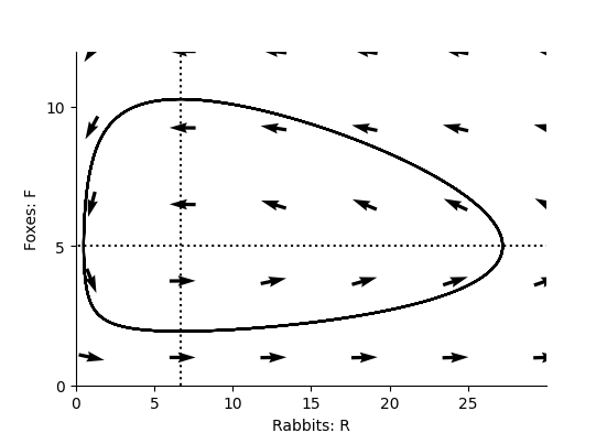
We can draw arrows to indicate the direction of change. To do this, we evaluate \(dR/dt\) and \(dF/dt\) for different values and plot them.
x = np.linspace(1, 30 ,6)
y = np.linspace(1, 12, 5)
X , Y  = np.meshgrid(x, y)
dX, dY = dXdt([X, Y])
#Make in to unit vectors.
M = np.hypot(dX,dY)
dX = dX/M
dY = dY/M

fig,ax=plt.subplots(num=1)
ax.quiver(X, Y, dX, dY, pivot='mid')
#Plot the rabbit equilibrium
ax.plot([-100,100],[a/b,a/b],linestyle=':',color='k')
#Plot the fox equilibrium
ax.plot([d/c,d/c],[-100,100],linestyle=':',color='k')
plotPhasePlane(ax,R,F)
Parker describe’s the cycle
Here is how Professor Parker sums up what we have learnt in Santa Fe.

Describing the cycle
Although we can’t find an explicit solution to the Lotka-Voltera model in terms of time, we can use a trick that Lotka described in an article he wrote in 1920 <https://www.pnas.org/doi/full/10.1073/pnas.6.7.410to>. By dividing the rabbit equation by the fox equation he got
We can then rearrange this equation to get
Integrating both sides of this equation we get
where \(C\) is the constant of integration. This last equation tells us a relationship that must always hold between rabbits and foxes. To understand what the relationship implies, imagine the equation above was simply \(Y+X=C\) instead. This would imply the total number of rabbits and foxes is equal to C=10. So, if \(C=10\) then we could have \(Y=3\) foxes and \(X=7\) rabbits (because 3+7=10), or 6 foxes and 4 rabbits (because 6+4=10), but we couldn’t have \(Y=6\) foxes and \(X=7\) rabbits (because 6+7≠10). In our case, the relationship in the equation is more complicated, involving logarithms, but the idea is the same: for any particular value of C all values of \(R\) and \(F\) must obey the equation
This is the case for the cycle we created in our numerical solution above. Every point on the predator-prey cycle fulfills the condition above.
Here is how Lotka presented his result in the original article.

While Lotka didn’t have a computer to simulate the equations, he could see using this argument that the cycles would remain finite. Neither the prey or predator populations would increase without bound.
Total running time of the script: ( 0 minutes 0.362 seconds)